The downloaded binary packages are in
/var/folders/1j/qb3qtyq94gxfdcs5wx9wt4zr0000gn/T//RtmpRnOu7G/downloaded_packageseasygenetics
2018-04-24
Navigating through the package
The package is a GUI dimension of basic functions that are used for genetic data analysis
Navigating through the package requires minimal or no coding exposure
In the documentation, we have made sure to present the instructions in a way as easy as possible.
Contents
- Introduction to
easygenetics - Installation
- GitHub
- Posit Connect Cloud
- User Interface
- List of Functions
- Using functions in easygenetics
- Significance of easygenetics
- Additional Details
- Session Info
- Contact Details
Introduction to easygenetics
easygeneticsis a front end genetic data analysis platform in R programming environment- It is a R package, consisting of functions which can be accessed and played with via a graphical interface
- The aim of this package is to create an easily accessible platform for non-statisticians and non-programmers to work on with minimal coding
- The user will have the minimum task of just loading the package and running the required function
- The input variables can be entered in the GUI, and results are available almost instantaneously, which improves the accessibility for non-programmers
Installation
- GitHub
The r package devtools is needed to install the easygenetics package from GitHub
devtools can be installed using
Then the easygenetics package can be installed using install_github() function from devtools package as below:
Installation
- Posit Connect Cloud
The Shiny app can be accessed using the link - easygenetics
The app is made using shiny package in R and hosted on Posit Connect Cloud
User Interface
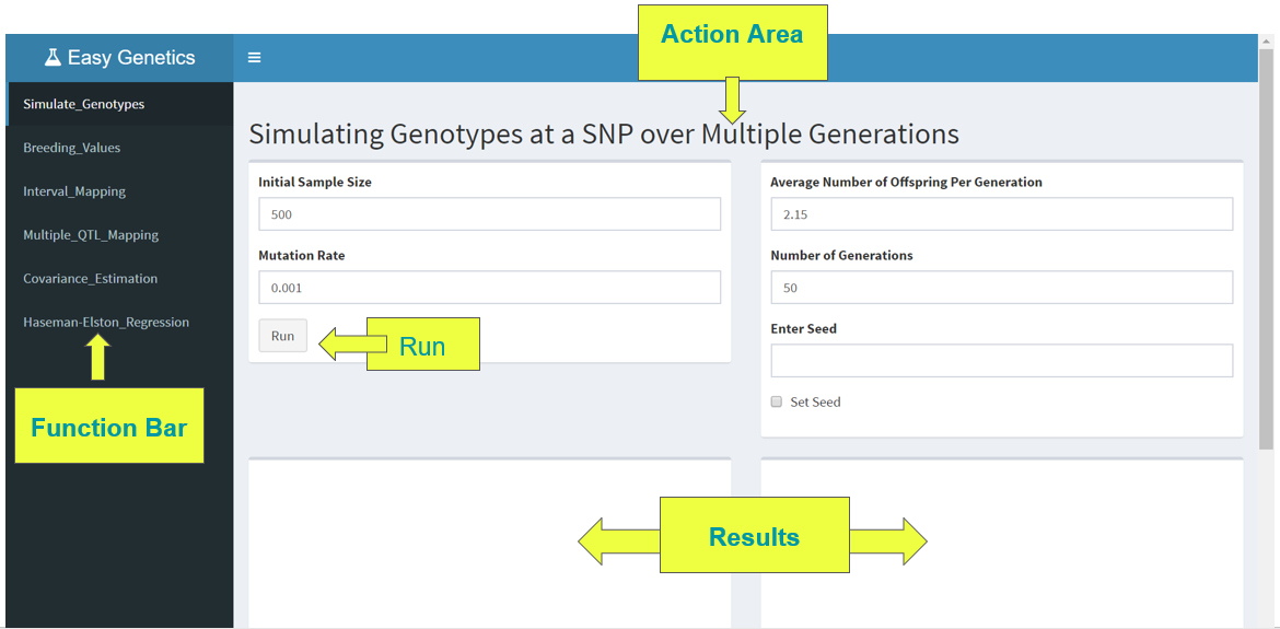
easygenetics User InterfaceThe Function Bar consists of the index of functions which makes it easier to access when you are using the package
The Action Area allows you to manipulate the parameters and observe and visualize the results parallely
The Results area allows you to visualize the results
The Run button lets you submit your values and observe the results
List of Functions
- Simulating Genotypes at a SNP over Multiple Generations :
Simulate_Genotypes() - Genotypic Values, Breeding Values, and Dominance Deviation Table :
Breeding_Values() - Interval Mapping :
Interval_Mapping() - Multiple QTL Mapping :
Multiple_QTL_Mapping() - Simulating Genotype of Parent by Child- Estimating Covariance :
Covariance_Estimation() - Haseman-Elston Regression :
Haseman-Elston_Regression()
Simulate_Genotypes()
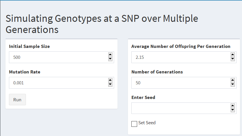
The function located on the first tab titled Simulate_Genotypes() is used to simulate genotypes at a SNP over multiple generations with the assumption that the mutation only happens one way
Input
- The arguments that are required in order for this function to properly run is the
initial sample size,mutation rate,average number of offspring per generationandnumber of generations - The
Enter Seedis a numeric value that allows the results to be reproducible - All of the required arguments needed in order for the function to work are numeric values
- The
initial sample sizeis the starting population size at the beginning of the simulation - The
mutation rateis the frequency of the target mutation in one gene over time - The
average number of offspring per generationis the mean growth in each generation
Output
- The output of this function produces two plots
- The first plot shows the
growth in population size over generation - The second plot provides the
allele frequency over generation
- The first plot shows the
These plots are both determined by the user’s arguments that are defined above.
Simulate_Genotypes()
Simulate_Genotypes()Breeding_Values()
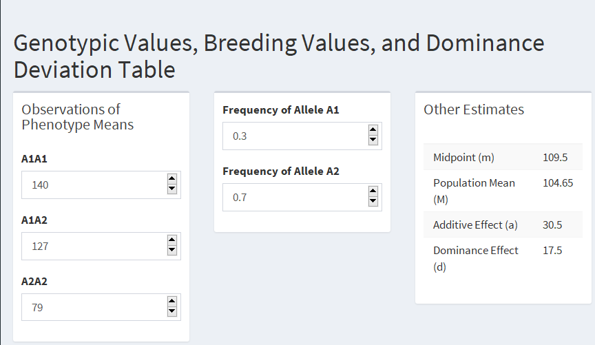
The second tab is titled Breeding_Values(), which calculates values based on the inputted arguments
Input
- The inputs for this function are all numeric
A1A1is the number of observations of the phenotypic means of the specified homozygous genotypeA1A2is the number of observations of the phenotypic means of the heterozygous genotype, andA2A2is the number of observations of the phenotypic means of the specified homozygous genotype- The
Frequency of Allele A1is the rate at which allele A1 occurs, and theFrequency of Allele A2is the rate at which allele A2 occurs
Output
The output of this function provides
- Table that includes
midpoint (m),population mean (M),additive effect (a),dominance effect (d) - Another table with the
frequency,genotypic value,breeding valueanddominance deviation of each genotype
- Table that includes
Breeding_Values()
Breeding_Values()Breeding_Values()
Glossary
Midpointis the middle value of the phenotypic means between the two homozygous genotypesExpected mean phenotypeis calculated using the additive effect and dominance effect , whereadditive effectis the distance between the midpoint and the phenotypic means of the homozygous genotypes, anddominance effectis the distance between the midpoint and phenotypic mean of the heterozygous genotype
Population meanis calculated from theadditive effect,dominance effectand thefrequencies of each genotypeFrequencyis the rate at which each genotype occursGenotypic valueis theadditive effectanddominance effectestimatesBreeding valueis the sum of average effects of the allelesDominance Deviationis the difference between genotypic value and breeding value
Interval_Mapping()
Interval_Mapping() is the function located on the third tab of the app - Interval mapping is currently the most common method used for QTL mapping - Its used by assuming the presence of a single QTL, and estimates the QTL position between two chosen markers after considering each locus one at a time
Input and Output
The
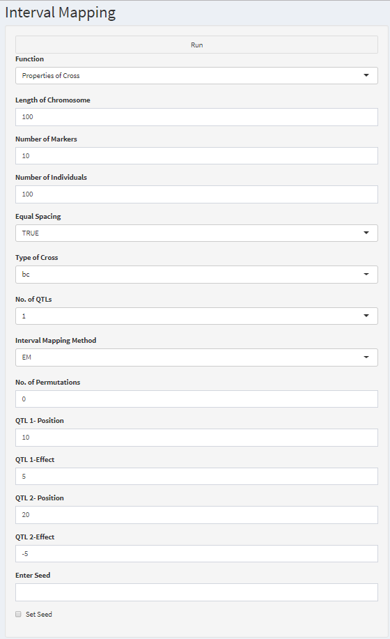
Enter Seedis a numeric value that allows the results to be reproducibleFunctionis a select list input with the optionsProperties of CrossPlotLOD Thresholds, andLOD Intervals
The default in this list is
Properties of Crossand the output changes depending on this selectionIf
Properties of Crossis selected and all the other parameters are entered and selected, the output displays the summary of a data simulation for a QTL experiment. This summary includes information such as thetype of cross,number of individuals,number of phenotypes,total markers,percent genotypedand so onIf
Plotis selected and all the other parameters are entered and selected, the output displays an interval mapping plot. Depending on what is selected under Interval Mapping Method determines what plot is displayedIf the option
LOD Thresholdsis selected, the output provides the summary of a genome scan with a single QTL model. This includes the interval mapping threshold that shows which chromosome , position and LOD value where the LOD threshold is locatedSelecting
LOD Intervalunder Function produces an output that shows the LOD support interval for the chromosome
Interval_Mapping()
Input and Output
The output described above is determined based on the other parameters that the user provides
This includes the
length of chromosome, thenumber of markers, thenumber of individuals, thenumber of permutations, theposition of QTL1andQTL2and theeffect of QTL1andQTL2, which are all numeric valuesEqual Spacing,Type of Cross,No. of QTLsandInterval MappingMethod are all select list inputs due to the restrictions of the functionEqual Spacingprovides the option of TRUE or FALSE that determines the presence of equal spacing in the genetic map simulationType of Crossspecifies what kind of population to simulate, and has the option ofbcwhich stands for backcross andf2for intercross- The choices for
No. of QTLsare1and2due to function constraints Interval Mappingmethod is used to determine which plot is shown. The options for the different methods areEM,HK,EHKandAll
Interval_Mapping()
Interval_Mapping()Multiple_QTL_Mapping()
Multiple_QTL_Mapping() is the next function in the tab and is used for multiple QTL mapping by the Haley-Knott Regression
- The downside of mapping one QTL at a time is that a second QTL might be missed, or ghosted
- By performing multiple QTL mapping, more QTLs can be identified on the same chromosome
Input
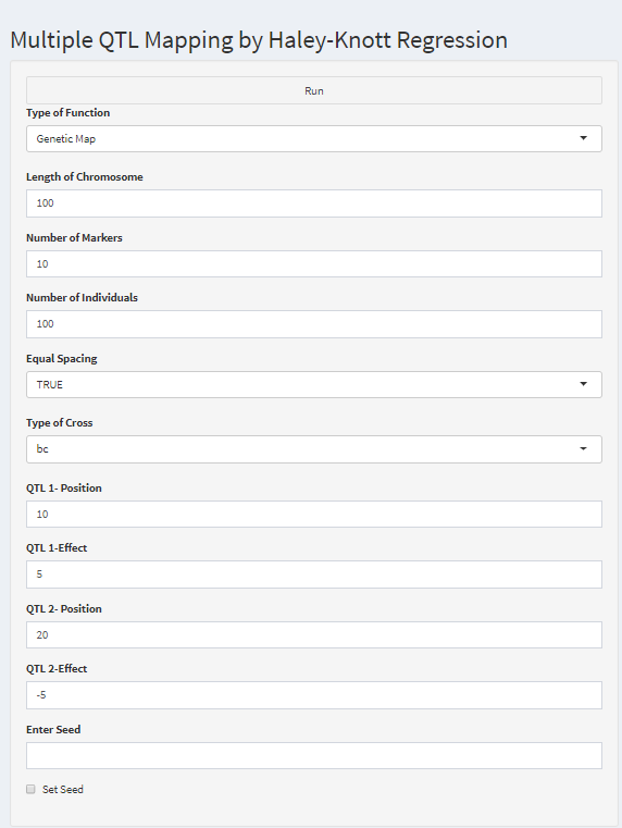
To execute this function, there are parameters that need to be set, which will be described below
- The
Enter Seedis a numeric value that allows the results to be reproducible - The
Type of Functionis a select list input with the options ofGenetic MapSingle QTLTwo QTLsHeat Map-Two QTLs ComparisonTwo QTLs ComparisonComposite Interval Mapping
- The default is set to
Genetic Map
Multiple_QTL_Mapping()
Output
Depending on what is selected and what the other inputs are, determines the output displayed
- By selecting
Genetic Map, the output shows a plot marker map - The
Single QTLoption plots the LOD score for each map position in centimorgans of a single QTL, which is the QTL the user clarifies in QTL1. A summary of this using Haley-Knott regression is presented below the plot - The same output is shown for when
Two QTLsis selected, except now the method uses a two-QTL model - Choosing
Heat Map-Two QTLs Comparisonchanges the output into a heat map of the QTLs - With
Composite Interval Mappinga plot is given with the black curve representing single interval mapping where the QTLs are not clearly distinguished and the blue curve is the composite interval curve. Below the plot the LOD threshold of the composite interval curve is provided in summary.
The rest of the parameters are similar to the ones in the Interval_Mapping function. In order for the output to be present, there needs to be a numeric value entered into the length of chromosome , the number of markers , the number of individuals , the position of QTL1 and QTL2 , and the effect of QTL1 and QTL2. Equal Spacing has a choice between TRUE and FALSE that determines the presence of equal spacing in the genetic map simulation. Type of Cross has options bc for backcross and f2 for intercross to determine what kind of population to simulate.
Multiple_QTL_Mapping()
Multiple_QTL_Mapping()Covariance_Estimation()
- The
Covariance_Estimationfunction is used to estimate variance between a parent and offspring
Input
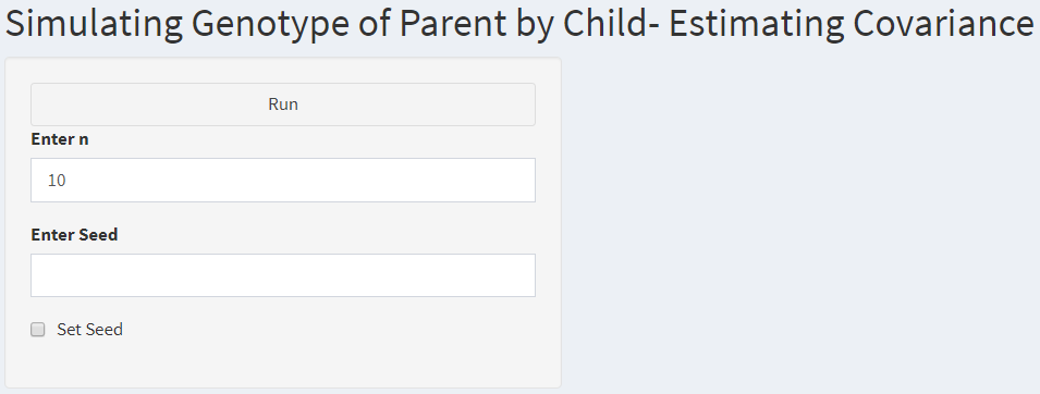
The user must specify the number of generations \(n\) as a numeric value under parameter
Enter nThe covariance is estimated through simulation, using a normal distribution to randomly generate the two parental allelic effects and a binomial distribution to randomly determine the transmitted allele. The transmitted allele assists in determining the offspring’s phenotype. Before estimating the covariance the appropriate errors are added to the parent and offspring, such as the environmental error.
The
Enter Seedis a numeric value that allows the results to be reproducible.
Output
The output displayed is the covariance estimation between parents and offsprings established from \(n\)
Covariance_Estimation()
Covariance_Estimation()Haseman-Elston_Regression()
The Haseman-Elston Regression function is used to obtain a series of plots which represent the relationship between the phenotypes of two siblings.For each sibling pair, the proportion of alleles IBD are determined at a given locus. The regression is done on squared difference between the sibling trait values on the proportion of alleles shared IBD. The variance component comes from genetic and environmental factors.
If \(y\)\(i\) denote the outcome variable for subject \(i\), then the Haseman-Elston regression model is-
\(y\)\(i\) = \(\mu\) + \(\alpha\)\(i\) + \(\alpha\)*\(i\) + \(\epsilon\)\(i\)
where \(\alpha\)\(i\) and \(\alpha\)* represents the additive genetic variance contribution from QTLs from inside and outside the interval. \(\alpha\), \(\alpha\)* and \(\epsilon\) are uncorrelated random errors, and the phenotypic variance is the sum of variance of these 3 random terms. The sum of \(\sigma_\alpha^2\) and \(\sigma_\alpha^{*2}\) is the total genotypic variance, whereas \(\sigma_\epsilon^2\) represents the error variance, which is the difference between the total variance and sum of genotypic and environmental variance.
Haseman-Elston_Regression()
Input
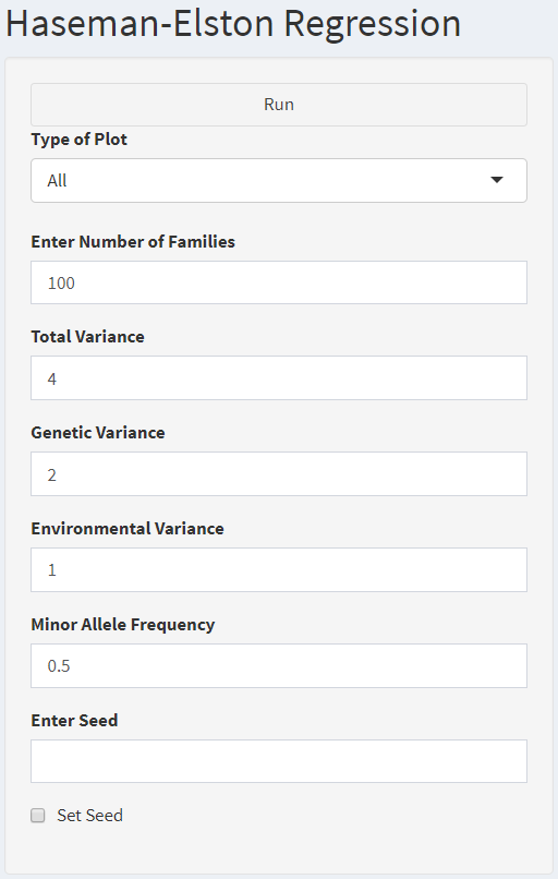
The
Enter Seedis a numeric value that allows the results to be reproducibleType of Plotis the select list input where we can select the type of plot we want in the result window. The options areHistogram of IBD,IBD vs Squared differences between phenotypes,Phenotype plot- Sibling 1 vs Sibling 2andPhenotype plot- Sibling 1 vs Sibling 2forIBD= 0,1,2. An additional option isAll, which shows all the above mentioned plots togetherNumber of Familiesis a numeric input variable which indicates the number of families on which the regression is to be performedTotal Variance,Genetic VarianceandEnvironmental Variancerepresent the Total Phenotypic Variance and the contribution of Genetic and Environmental component respectivelyMinor Allele Frequencyis the frequency of the minor allele in the population.
Output
The default output plot type is All , which produces all plots- Histogram of IBD , IBD vs Squared differences between phenotypes , Phenotype plot- Sibling 1 vs Sibling 2 and Phenotype plot- Sibling 1 vs Sibling 2 for IBD= 0,1,2. Histogram of IBD shows the frequency distribution of population which belongs to each IBD category. IBD vs Squared differences between phenotypes plots the squared difference between phenotypic values of siblings by the three IBD values- 0,1 and 2. Phenotype plot- Sibling 1 vs Sibling 2 shows the overall scatter plot of phenotypic values of sibling 1 and sibling 2. Phenotype plot- Sibling 1 vs Sibling 2 for IBD= 0,1,2 represent the subset of the overall phenotypic plot segmented by IBD values 0,1 and 2.
Haseman-Elston_Regression()
Haseman-Elston_Regression()